Optimization · Muon · LLM pretraining
How Muon Sublates the Edge of Stability
What survives at the edge—and what changes when updates become matrix-aware?
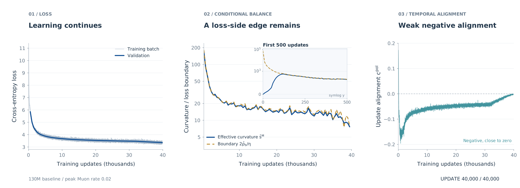
What does training at the edge of stability look like when the optimizer is Muon? Let’s start with a 130M language model. Watch the three panels below as training unfolds: the loss improves, the measured curvature approaches a loss-balance boundary, and consecutive update directions settle slightly below zero alignment.

 One clock for all three panels · early updates slowed
Figure 1 · Continued learning near a loss-side edge. The 130M baseline (peak Muon rate 0.02) tracks its conditional loss boundary while consecutive directions remain weakly negatively aligned. Loss describes complete Muon-plus-AdamW training; balance comes from Muon-only checkpoint probes. The alignment panel starts at step 0 and retains all recorded early updates; the main balance panel begins at step 500. The inset inside the middle panel shows updates 0–500 on a symmetric-logarithmic y-axis, including the slightly negative initial curvature. Faint paths show the complete trajectories for context; colored paths reveal the original observations without smoothing. Playback is slower during the first 500 updates. “Pause · show all data” displays the complete figure.
Start with the middle panel. The two curves track each other over much of training; the inset shows how this develops during the first 500 updates. Now look right: the direction cosine remains negative, but close to zero. The updates are nearly orthogonal, with a small opposing component. Meanwhile, the left panel shows continued learning.
How can a loss-balance edge coexist with so little directional reversal? To understand this picture, we will first revisit the familiar gradient-descent example, then see what changes when Muon transforms a matrix gradient. This will lead to two quantities that let us read the loss and direction panels separately. At the end, we will ask how these quantities might help us choose learning rates and batch sizes.
1. What is the Edge of Stability?
Imagine training a neural network with a fixed learning rate. We might expect training to stay in a region where every step decreases the loss. Yet full-batch gradient descent often does something more surprising: the loss fluctuates over short intervals while improving over longer ones, and the largest Hessian eigenvalue stays near the scale \(2/\eta\). This is the edge of stability (EoS) behavior documented by Cohen et al. (2021).
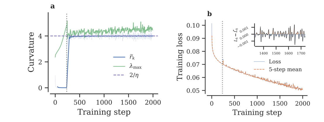
Figure 2 · Training keeps improving near the classical edge. Follow curvature toward the learning-rate scale, then compare the short-term loss fluctuations with the longer-term decrease. Full-batch GD, three-layer MLP, CIFAR-10, learning rate 0.5. Reproduced unchanged from Litman (2026), Figure 1, under CC BY 4.0.
Why does this particular scale appear? A single quadratic mode gives us a useful starting point.
Where does the scale 2/η come from?
For one scalar quadratic mode, \(L(x)=\lambda x^2/2\), GD gives
\[x_{k+1}=(1-\eta\lambda)x_k.\]The multiplier \(1-\eta\lambda\) determines whether this mode contracts or grows. For \(0<\eta\lambda<2\), its magnitude shrinks; above \(2\), it grows. At \(\eta\lambda=2\), the multiplier is \(-1\): the loss stays constant, consecutive updates reverse with equal magnitude, and the mode is marginally stable. This simple calculation explains the classical boundary scale.
How step size changes quadratic GD
Same loss, different step sizes. Each dot follows xₖ₊₁ = (1 − ηλ)xₖ on L(x) = λx²/2, with λ = 1.
ηλ = 0.8
Converges without oscillating
Strictly inside the boundary
ηλ = 1.8
Converges while oscillating
Oscillation alone does not imply an edge
ηλ = 2.0
Marginal: exact reversal
At the boundary by construction
ηλ = 2.2
Diverges while oscillating
Outside the boundary
Toy illustration. Curvature is fixed in all four panels. This does not show a neural-network trajectory discovering or tracking an edge; it only explains the scalar stability threshold. The boundary case is imposed through the step size.
Watch the mode at \(\eta\lambda=2\): each step lands on the opposite side at the same distance from the minimum. Loss neutrality and equal-magnitude reversal coincide here. Direction changes already occur above \(\eta\lambda=1\), so a negative cosine by itself does not identify this edge. At exactly one, the next gradient vanishes and its cosine is undefined.
A boundary is only the beginning
The quadratic example tells us where a local mode stops contracting. The neural-network experiment asks a further question: does training actually approach and remain near a boundary while continuing to learn? We need both the boundary calculation and the trajectory measurements to answer that question for Muon.
This distinction also connects two strands of earlier work. Wu, Ma and E (2018) study minima selected through linearized stochastic stability, while Cohen et al. study EoS behavior along training trajectories. Our starting point is the scalar GD mechanism above. We will now examine which of its connections survive a change in update geometry.
2. Muon changes relative update strengths
A matrix gradient can have very different strengths along its singular directions. Multiplying it by a learning rate scales all those strengths together. Muon changes their relative sizes.
In the diagram below, compare the image of the same input circle under the gradient and under its polar factor. A strong singular direction stretches the gradient’s image more than a weak one. The polar map gives every active singular direction unit strength. Its compact SVD makes that operation explicit:
\[\widehat G_k=U_r\Sigma_rV_r^\top, \qquad P_k=\operatorname{Pol}(\widehat G_k)=U_rV_r^\top, \qquad W_{k+1}=W_k-\eta P_k.\]It keeps the active left and right singular vectors and replaces their nonzero singular values by one. Multiplying the whole gradient by one scalar would leave those values in the same proportions. Muon changes the proportions. Zero singular directions remain zero.
A matrix acts on directions
Same singular directions. Different relative strengths.
Follow matching colored points as the same unit input circle is mapped by G and its exact polar factor.
Raw gradient G
Singular values
Exact polar direction P
Singular values
\(W_{k+1}=W_k-\eta P_k.\) The update is transformed; the weight matrix itself is not being orthogonalized.
What does the actual five-step Newton–Schulz approximation do?
The transform starts from the Frobenius-normalized gradient and applies the Muon quintic to each singular value:
Inner iteration / 5
Singular values
These are iterations inside one matrix transform, computed in double precision. They are not training steps. The finite quintic does not return exactly unit singular values; a zero singular value stays zero.
Figure 3 · Muon changes the map's relative strengths. The two main panels share one scale and use the same colored input points. Exact polar normalization retains the active singular directions and equalizes their singular values. Setting σ₂ to zero shows the canonical partial-polar case. The expanded view computes actual NS iterations rather than interpolating shapes.
Interactive presentation inspired by Mishra's matrix-map lab and Newton–Schulz notes; independent implementation. See also Bernstein's derivation.
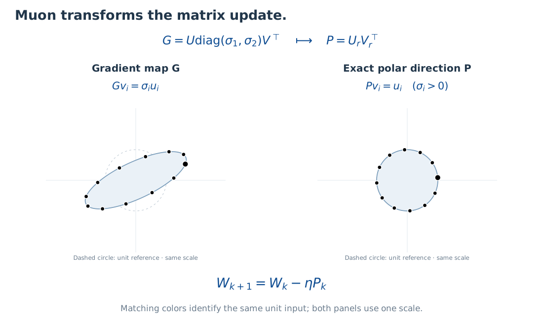
Try changing one singular value in Figure 3. The gradient’s shape changes, while the exact polar map keeps unit strength along the active directions. This is the geometric change that prevents us from carrying the scalar GD picture over unchanged.
Why does this transformation still give a descent direction? With a spectral-norm step budget, it has a steepest-descent interpretation: with a spectral-norm step budget, the polar direction maximizes first-order descent,
\[P\in\operatorname*{arg\,max}_{\|D\|_2\leq1}\langle\widehat G,D\rangle_F, \qquad \langle\widehat G,P\rangle_F=\|\widehat G\|_*.\]Here \(\|D\|_2\) is the matrix spectral norm, and \(\|G\|_*\) is the nuclear norm. This is why a nuclear norm appears in the loss identity below. Our controlled experiments use SVD-polar directions; LLM runs use the practical five-step Newton–Schulz approximation, NS-5, without momentum.
Why does the nuclear norm appear?
Write \(G=U_r\Sigma_rV_r^\top\). For any \(\|D\|_2\leq1\), each active singular pair satisfies \(\lvert u_i^\top Dv_i\rvert\leq1\). Consequently,
\[\langle G,D\rangle_F=\sum_{i=1}^{r}\sigma_i u_i^\top Dv_i \leq\sum_{i=1}^{r}\sigma_i=\|G\|_*.\]Taking \(D=U_rV_r^\top\) attains equality. The linearized loss change of \(-\eta D\) is therefore minimized by the polar direction under this norm budget. This argument concerns the exact no-momentum direction; an approximate transform does not automatically inherit every exact-polar property. See Bernstein’s derivation for the broader layer-geometry perspective.
For a differentiable optimizer map \(F(W)=W-\eta T(\nabla L(W))\),
\[DF(W)=I-\eta\,DT(G)\circ\nabla^2L(W).\]GD has \(T=\operatorname{Id}\). A nonlinear matrix transform adds its own local response, with care required at rank changes. This explains why the GD mechanism cannot simply be transferred; it is not a stochastic stability theorem for Muon.
3. Why the classical coupling splits
We can now ask two concrete questions. Will the current step lower the loss? And how will the next update align with this one? The first uses the direction we take now; the second also depends on the direction produced at the next state.
Read the schematic from left to right. The scalar GD example ties loss balance to an equal-magnitude reversal. For Muon, we need a loss-side coordinate and a direction-side coordinate to describe the state.
From one mechanism to two diagnostics
Classical coincidence becomes a two-coordinate question.
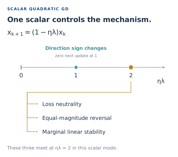
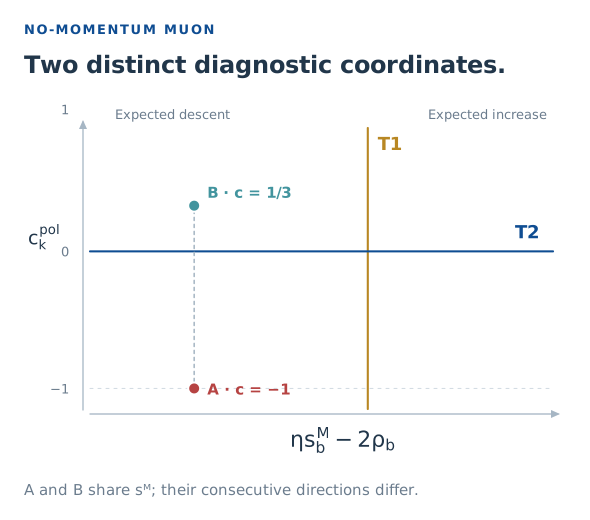
The GD calculation concerns one scalar quadratic mode. The Muon panel is a diagnostic coordinate map, not a perturbation-stability phase diagram or a claim that every point is attainable. A/B are the exact full-batch construction in Figure 5, with ρ = 1. At ηλ = 1, the GD next update vanishes and its cosine is undefined.
T1: the conditional loss‑neutral boundary
To answer the loss question, imagine pausing training at \(W_k\) and trying fresh minibatches of size \(b\). How much useful descent survives the sampling and polar transformation? With nonzero full gradient \(G_k=\nabla L(W_k)\), define coherence
\[\rho_b=\frac{\mathbb E_b\langle G_k,P_k\rangle_F}{\|G_k\|_*}.\]It measures how much first-order descent is retained after sampling and polar normalization. An unbiased sampled gradient does not guarantee an unbiased polar direction. Exact-polar duality gives \(\rho_b\in[-1,1]\).
A finite step also pays a curvature cost. We summarize that cost by an effective curvature \(s_b^M\) defined from the loss remainder. The competition between descent and curvature gives the exact identity
\[\mathbb E_b[L(W_{k+1})-L(W_k)\mid W_k] =\frac{\eta^2\|G_k\|_*}{2}\left(s_b^M-\frac{2\rho_b}{\eta}\right).\]Read the bracket: negative means expected descent, zero means balance, positive means an expected increase. T1 is therefore \(s_b^M=2\rho_b/\eta\). Full-batch exact-polar Muon has \(\rho_{\mathrm{full}}=1\) and recovers the scale \(2/\eta\). The effective curvature is a normalized directional loss remainder, not the maximum Hessian eigenvalue.
Deriving the conditional loss identity
Let the finite-step remainder be
\[r_k(P)=L(W_k-\eta P)-L(W_k)+\eta\langle G_k,P\rangle_F.\]Define
\[s_b^M(W_k;\eta)=\frac{2\mathbb E_b r_k(P_k)}{\eta^2\|G_k\|_*}.\]Rearranging the remainder and taking conditional expectations gives
\[\mathbb E_b\Delta L=-\eta\mathbb E_b\langle G_k,P_k\rangle_F +\mathbb E_b r_k(P_k) =-\eta\|G_k\|_*\rho_b+\frac{\eta^2\|G_k\|_*}{2}s_b^M.\]Factoring yields the displayed identity. It requires continuous differentiability, nonzero \(G_k\) and finite expectations, not a second-order Taylor approximation. With additional second-order smoothness, the small-step limit at a fixed state is
\[s_b^M\longrightarrow\frac{\mathbb E_b\langle P_k,H_k[P_k]\rangle_F}{\|G_k\|_*}.\]The equality defines the conditional boundary; it does not prove that training stays there. In practical multi-block probes, numerical direction normalization and the finite reference objective follow the paper’s experimental protocol rather than an ideal single-matrix calculation.
T2: the temporal-orthogonality boundary
Now turn to the direction question. Compare the current update with the next one using their cosine. For two nonzero consecutive directions,
\[c_k^{\mathrm{pol}}=\frac{\langle P_k,P_{k+1}\rangle_F}{\|P_k\|_F\|P_{k+1}\|_F}.\]T2 is the sign boundary \(c_k^{\mathrm{pol}}=0\). Positive means acute alignment; negative means obtuse alignment and partial cancellation relative to same-direction steps. A discrete trajectory can cross the sign boundary without attaining zero. A negative cosine alone proves neither a two-step return nor local perturbation stability.
In Figure 4, follow the two arrows: a positive cosine means they reinforce, zero means they are orthogonal, and a negative cosine means they oppose in part. Complete reversal is the special endpoint, not the meaning of every negative value.
From angle to motion
A negative cosine can still take you forward.


Figure 4 · Read alignment through two actual displacements. Each second arrow starts where the first ends. All steps have equal length. Only the equal, exactly opposite pair returns to the start; its red arrow is offset slightly for visibility.
For GD the direction-sign boundary is tied to a directional secant response of \(1/\eta\). For exact full-batch Muon, the corresponding value is geometry-dependent, \(\vartheta_k/\eta\). T1 and T2 are loss and direction diagnostics, not two interchangeable linear-stability criteria.
From direction cosine to two-step motion and the secant boundary
Let \(\Delta_k=W_{k+1}-W_k=-\eta_kP_k\). Then
\[\|W_{k+2}-W_k\|_F^2=\|\Delta_k\|_F^2+\|\Delta_{k+1}\|_F^2 +2\|\Delta_k\|_F\|\Delta_{k+1}\|_F c_k^{\mathrm{pol}}.\]At \(c=-1\), Cauchy–Schwarz gives proportional opposite directions. Exact nonzero polar factors both have operator norm one, so the proportionality factor is one. At fixed rate this yields \(P_{k+1}=-P_k\) and \(W_{k+2}=W_k\). For implemented NS-5 directions or unequal rates, opposite directions alone need not imply equal displacement lengths.
For full-batch exact-polar Muon, define
\[\bar s_k^M=-\frac{\langle P_k,G_{k+1}-G_k\rangle_F}{\eta\|G_k\|_*}, \qquad a_k=\frac{\|G_{k+1}\|_*}{\|G_k\|_*},\qquad r_k=\operatorname{rank}(G_k).\]Separate the next gradient into its mean singular strength and residual:
\[R_{k+1}=G_{k+1}-\frac{\|G_{k+1}\|_*}{r_{k+1}}P_{k+1}, \qquad \vartheta_k=1-\frac{\langle P_k,R_{k+1}\rangle_F}{\|G_k\|_*}.\]Using \(\|P_k\|_F^2=r_k\) gives
\[\bar s_k^M=\frac{\vartheta_k-a_k\sqrt{r_k/r_{k+1}}\,c_k^{\mathrm{pol}}}{\eta}.\]Thus \(c_k^{\mathrm{pol}}=0\) iff \(\bar s_k^M=\vartheta_k/\eta\), and negative cosine corresponds to a larger secant response. The coefficient \(\vartheta_k\) need not be one. This is an exact relation for a given step, not a universal curvature-only predictor. Loss curvature \(s_k^M\) and secant response \(\bar s_k^M\) agree for constant Hessian, but generally weight curvature along the update segment differently. See paper Appendix A.3.
Same loss curvature, different next directions
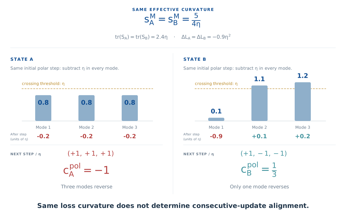
Can the same loss curvature really produce opposite signs of alignment? Take the paper’s \(X=I_3\) example and restrict \(W-W_{\min}\) to a diagonal matrix with signed coordinates \(e_1,e_2,e_3\). The loss becomes \(L=\tfrac12\sum_i e_i^2\), so the three modes have identical quadratic bowls. Initially all coordinates are positive: exact polar Muon therefore takes the same step, \(\Delta_k=-\eta I_3\), in both states.
Each mode moves left by η, regardless of its initial strength. In A, every coordinate overshoots zero and the next step reverses all three directions. In B, just one coordinate overshoots; the other two keep moving left. This makes the difference in alignment visible.
The key comparison is equal effective curvature with different update alignment. T1 depends on the sum of the initial strengths, or trace. Alignment depends on how many modes cross zero. Two initial points on the same plane \(e_1+e_2+e_3=2.4\eta\) can therefore have the same effective curvature and different next directions.
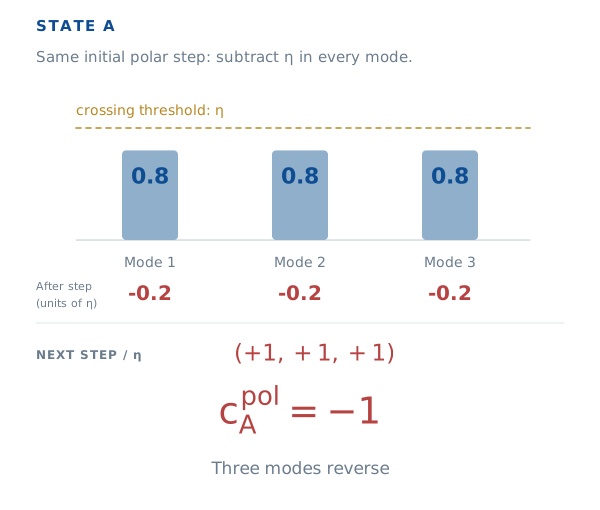
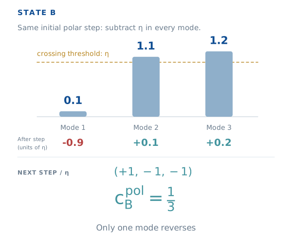
Same effective curvature. Different consecutive-update alignment.
View the mode-by-mode quadratic construction
State A


State B


Figure 5 · The same s does not determine c. Initial strengths are compared to the same η crossing threshold. The shared trace fixes the effective curvature and loss increment, while three versus one mode reversals give c = −1 and c = 1/3. The full derivation and optional mode sections explain this exact X = I₃ construction.
Working through the matrix counterexample
Consider \(L(W)=\tfrac12\|WX-Y\|_F^2\) with \(XX^\top\succ0\), \(m\geq d\), a full-column-rank gradient and nonsingular \(S_k-\eta XX^\top\), where \(G_k=P_kS_k\) and \(S_k=(G_k^\top G_k)^{1/2}\). The affine gradient gives
\[G_{k+1}=G_k-\eta P_kXX^\top=P_k(S_k-\eta XX^\top).\]Because \(P_k^\top P_k=I_d\), its next stretch and polar factors are
\[S_{k+1}=\lvert S_k-\eta XX^\top\rvert, \qquad P_{k+1}=P_k\operatorname{sign}(S_k-\eta XX^\top).\]The absolute value and sign act eigenvaluewise. The quadratic loss expansion yields
\[\Delta L=-\eta\operatorname{tr}(S_k)+\frac{\eta^2}{2}\|X\|_F^2, \qquad s_k^M=\frac{\|X\|_F^2}{\operatorname{tr}(S_k)}.\]If \(n_-\) counts negative eigenvalues of \(S_k-\eta XX^\top\),
\[c_k^{\mathrm{pol}}=\frac{\operatorname{tr}\operatorname{sign}(S_k-\eta XX^\top)}{d} =1-\frac{2n_-}{d}.\]Take \(X=I_3\) and either \(S_k=\eta\operatorname{diag}(0.8,0.8,0.8)\) or \(S_k=\eta\operatorname{diag}(0.1,1.1,1.2)\). Both traces are \(2.4\eta\), so both have \(s_k^M=5/(4\eta)\) and \(\Delta L=-0.9\eta^2\). Their shifted spectra have three and one negative eigenvalues, giving \(c=-1\) and \(c=1/3\). Equal loss curvature therefore does not determine alignment. See paper §2.3 and Appendix A.2.
What theory says about approaching the loss boundary
There is also a trajectory constraint. For full-batch exact-polar Muon at fixed rate on a lower-bounded objective, if the cumulative active-step weight \(\sum_k\eta^2\|G_k\|_*\) diverges, effective curvature cannot eventually stay a fixed distance below \(2/\eta\):
\[\limsup_{k\to\infty:G_k\ne0}s_k^M\geq\frac{2}{\eta}.\]This constrains curvature visits. Persistent tracking under stochastic NS-5 training remains an empirical finding to examine next.
Why curvature cannot stay uniformly below the boundary
Suppose all sufficiently late active steps satisfy \(s_k^M\leq2/\eta-\delta\) for some \(\delta>0\). Full-batch coherence is one, so the loss identity gives
\[L(W_{k+1})-L(W_k)\leq-\frac{\delta}{2}\eta^2\|G_k\|_*.\]Summing these increments would send loss to negative infinity if the cumulative weight diverges, contradicting the lower bound. Hence the limsup bound. It does not establish attraction, persistent tracking, or a temporal cosine condition. See paper Appendix A.1.
4. Do the diagnostics separate along training?
The example shows why one quantity cannot determine the other. Let’s now follow both during training. We begin with small networks, where we can vary the batch size, before returning to the language-model run that opened this article.
Controlled networks: batch size matters, and the order can swap
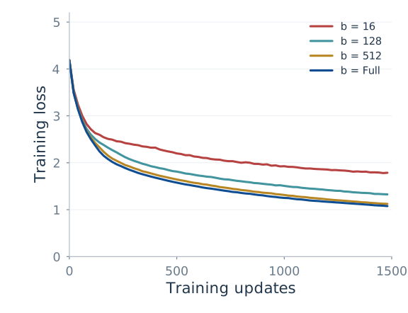
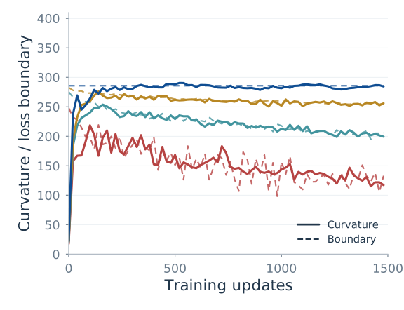
Read Figure 6 in pairs: compare loss balance with direction alignment for the same network and batch size. Then use Figure 7 to see which event happens first.
Loss
Loss balance
Consecutive directions
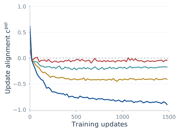
Figure 6 · Follow one batch size across the three panels. Exact SVD-polar Transformer at fixed rate 0.007. Larger batches show more negative alignment. The plotted vertices and batch labels are retained from the supplied vector PDFs.
Small batches remain closer to orthogonality; larger batches produce more negative alignment in these runs. The displayed full-batch global measurements approach coherent reversal without reaching \(-1\).
MLP
CNN
Transformer
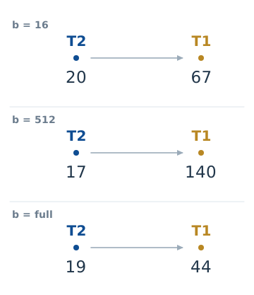
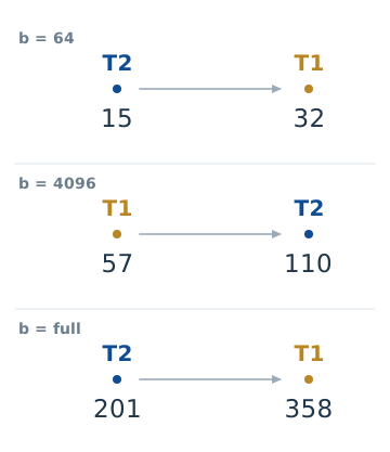
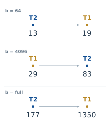
Figure 7 · The event order can swap. Each row reads from earlier to later. Numbers are the exact first qualifying steps in the supplied PDFs. Connecting lengths do not encode elapsed time. For MLP/CNN, T2 comes first at b = 64 and T1 comes first at b = 4096.
Compare the original event times on numeric axes
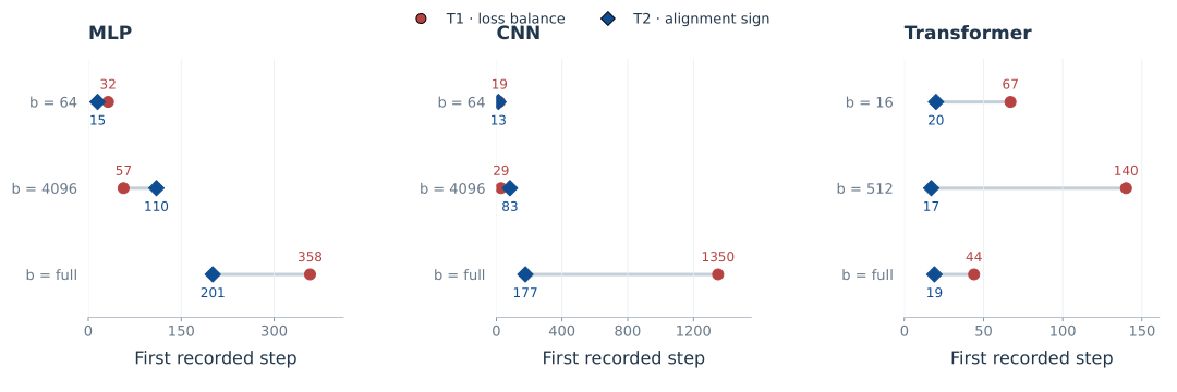
In the displayed event panels, T2 precedes T1 at batch 64 in the MLP and CNN; at batch 4096, T1 precedes T2. This illustrates their different responses along training. Unequal event times alone are not the proof of separation: even a scalar GD mode changes direction before loss balance. The matrix counterexample above supplies that proof.
LLMs: a loss boundary with weak negative alignment
The LLM runs use no-momentum NS-5 on Muon blocks and AdamW on auxiliary parameters. Their empirical diagnostics complement the exact-polar analysis; they do not make the approximation identical to the theoretical update.
| Experiment | Configuration | What to look for |
|---|---|---|
| 22M checkpoint branches | Batch 16 for rate interventions | Loss-change signs can switch while cosines stay negative |
| 130M training | Batch 32; sequence length 4096; about 5.23B tokens | Conditional boundary tracking and weak negative global alignment |
| 1B training | Batch 512; sequence length 4096; about 20B tokens | More negative alignment with improving loss; T1 was not measured |
Return to Figure 1 at the top. We can now read it more precisely. The middle panel concerns the conditional loss-neutral boundary, T1. The right panel measures temporal alignment relative to the orthogonality boundary, T2. Tracking the first does not require an approach to \(c=-1\) in the second. The left panel shows that learning continues throughout this directional regime.
Across four peak-rate runs, full-horizon cosine medians range from approximately \(-0.048\) to \(-0.032\). The central empirical pattern is sustained negative alignment close to orthogonality, together with continued learning.
The loss measurements have different scopes. Boundary tracking comes from finite-reference, Muon-only checkpoint probes. Validation improvement comes from complete Muon-plus-AdamW training. A near-zero conditional probe increment does not mean that the full run has stopped learning.
What changes when updates carry memory?
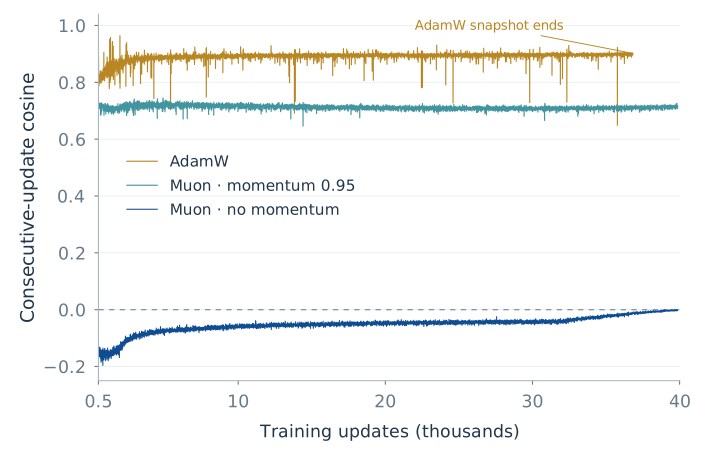
Does the weak negative alignment persist when the optimizer carries memory? Our additional 130M runs show a different directional picture: Muon with momentum 0.95 and AdamW both maintain positive alignment between consecutive updates.
Over the common window from updates 500 to 36,827, their mean global cosines are approximately 0.712 and 0.891, respectively. Every recorded global cosine is positive in both runs. The positive sign also persists in all 12 layers and all 84 individual matrix blocks, so it is not an artifact of averaging positive and negative blocks together.
130M · Optimizer memory
Positive alignment with momentum and AdamW
Global alignment through training
The positive sign persists across layers
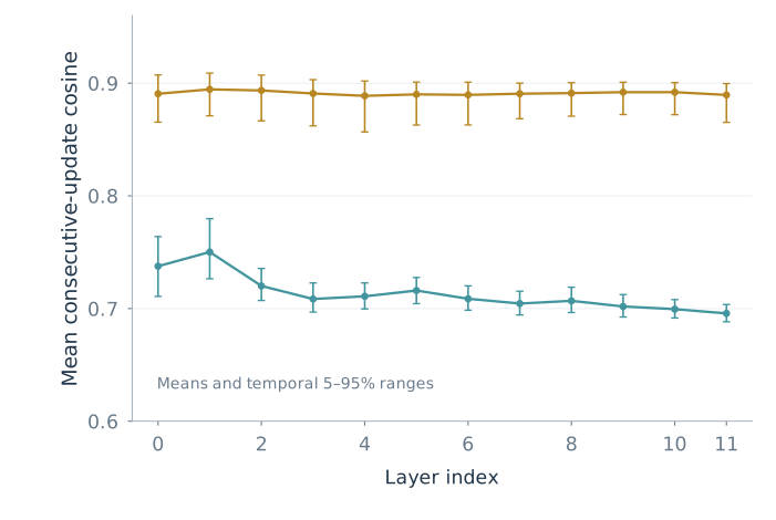
Figure 8 · Optimizer memory accompanies persistent positive alignment. The additional 130M runs use Muon with momentum 0.95 and Nesterov updates, or AdamW with β₁ = 0.9 and β₂ = 0.95. Every recorded global, layer-level and individual matrix-level cosine is positive in both runs. The right panel summarizes the common window from updates 500 to 36,827: dots are means and bars are temporal 5–95% ranges, not confidence intervals. The AdamW trajectory ends at its available snapshot.
The intuition is that a momentum update inherits directional information from earlier steps. Consecutive updates reuse part of the same gradient history, making persistent positive alignment natural even as fresh minibatches change. AdamW also carries a moving average of past gradients. This contrasts with the weakly negative, nearly orthogonal directions of the no-momentum Muon run in Figure 1: optimizer memory adds temporal persistence to the directional picture.
5. Change the learning rate at the same checkpoint
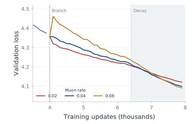
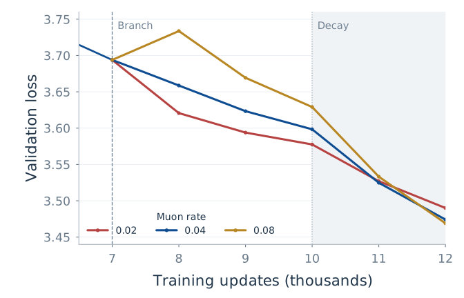
So far, we have watched quantities evolve together. What happens if we deliberately change the learning rate at a shared checkpoint? If loss balance and directional alignment contain different information, a change in one need not imply the same change in the other. We branch from 0.04 to 0.02, 0.04 or 0.08, keeping each model’s batch size and auxiliary AdamW schedule fixed. The branch points are step 4000 for 22M and step 7000 for 130M.
For 22M, the one-step conditional probes at step 4000 give:
| Muon rate | Conditional loss increment | 95% probe interval | Later mean cosine |
|---|---|---|---|
| 0.02 | −0.01967 | [−0.01999, −0.01936] | −0.064 |
| 0.04 | −0.00026 | [−0.00138, 0.00086] | −0.100 |
| 0.08 | +0.15219 | [0.14650, 0.15789] | −0.117 |
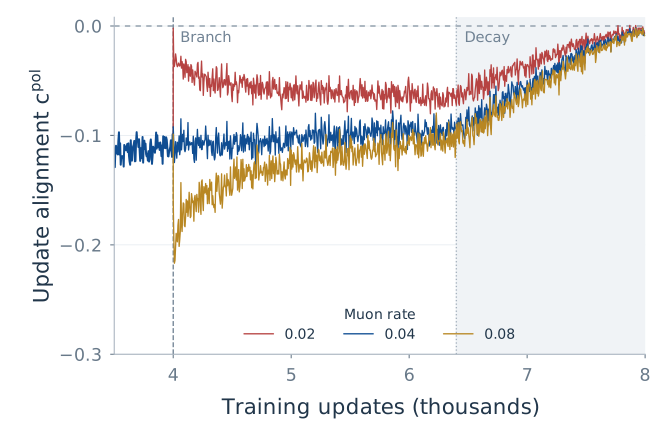
The expected loss response crosses from decrease to increase, while later alignment remains negative in all three branches. The middle interval contains zero; the smaller and larger rates fall on opposite sides of the loss boundary.
The columns refer to different horizons. Intervals come from eight paired one-step probes at one state, not across-seed uncertainty. Cosine means summarize 280 recorded pairs per branch during steps 5000–6399, with no reported intervals. The 130M rate branches have no conditional T1 probes.
22M · Branch from the same state at step 4000
Validation loss
Consecutive directions
130M · Branch from the same state at step 7000
Validation loss
Consecutive directions
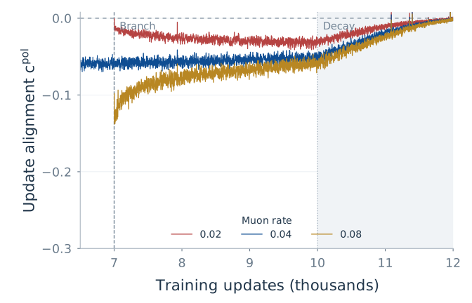
Figure 9 · The same intervention, viewed through loss and direction. Rows are model sizes; columns are diagnostics. Dashed vertical markers locate the branch; the grey region marks decay. Curves are redrawn from the supplied CSV/JSONL files without smoothing. These trajectories differ from the one-step conditional probes in the table.
Rate changes initially shift alignment, which then tends back toward its pre-change value. Both displayed continuations also enter learning-rate decay, so the later response reflects the schedule as well as the intervention. Some larger-rate branches also improve later validation loss. These observations motivate schedule research, but they do not establish a rule to raise the rate whenever cosine is near zero.
6. What do noise, layers and scale add?
The global cosine leaves several questions open. Do all layers behave alike? Is near orthogonality simply minibatch randomness? Does the pattern persist at larger scale? We can address each by changing what we measure.
A global average hides structure
First, look inside the model. In Figure 10, compare the key/value blocks with query blocks, then follow their alignment over time. The coherence curves below ask how the loss-side signal changes when we increase the probe batch.
Where is alignment most negative?
How does alignment evolve?
Larger probe batches retain more coherence
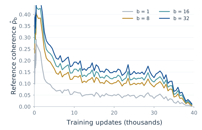
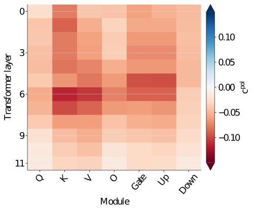
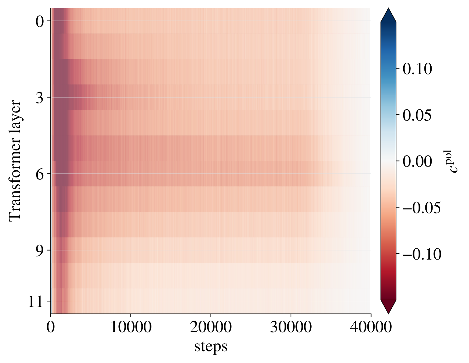
Figure 10 · A global average hides structured behavior. 130M baseline, peak rate 0.02. The heatmaps retain the supplied measured cells and original color scales centered at zero. Coherence is redrawn from the supplied checkpoint-probe data.
The module medians locate stronger negative alignment; the temporal heatmap shows its evolution; the coherence curves below show how probe sampling affects the loss-side signal. Middle-layer key/value matrices differ from many query matrices, and larger probe batches generally strengthen reference coherence. A global cosine near zero should therefore be read alongside the underlying layers and modules.
Is near orthogonality just minibatch randomness?
A frozen-state test helps distinguish sampling dispersion from temporal feedback. At a fixed checkpoint, compare independent minibatch directions without advancing the model. Then compare this with consecutive directions along the training trajectory.
Resample directions at the same checkpoint.
Compare directions at consecutive states.
Seed 2026
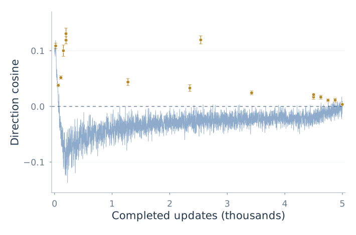
Seed 1337
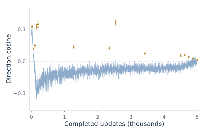
Figure 11 · Sampling dispersion and temporal feedback leave different signs. Tiny Transformer, batch eight. Gold points compare independent minibatch directions at one frozen state; vertical bars retain the original 95% delete-one-batch jackknife intervals. The blue trace compares consecutive directions along training. Both seeds share the same axes. No smoothing or continuous uncertainty band is added.
This supports sampling dispersion as a source of weak alignment and changes in the model state as a source of negative bias. Both Muon and AdamW change that state, so this test cannot assign the feedback to either optimizer alone.
At 1B, loss still improves despite stronger cancellation
Finally, Figure 12 repeats the loss-and-direction view at 1B scale. The cosine is more negative in this configuration, while the loss continues to improve. The layer traces show how broadly this directional behavior appears.
Learning continues at 1B
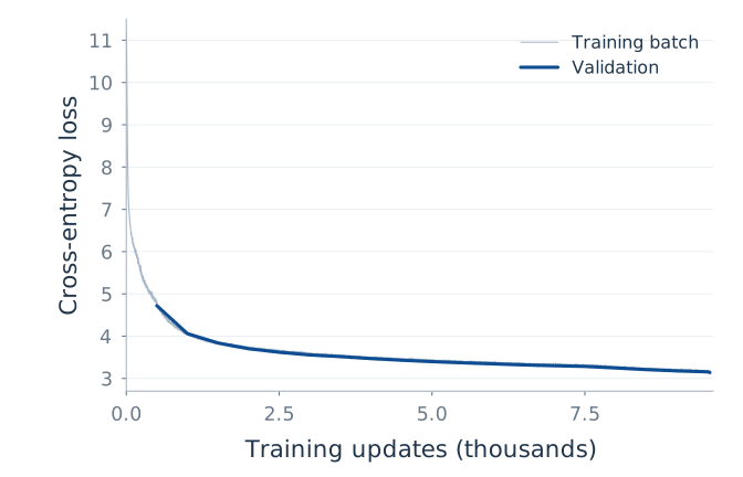
Stronger negative alignment
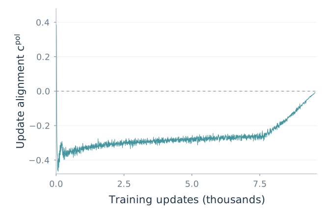
Layers follow different trajectories
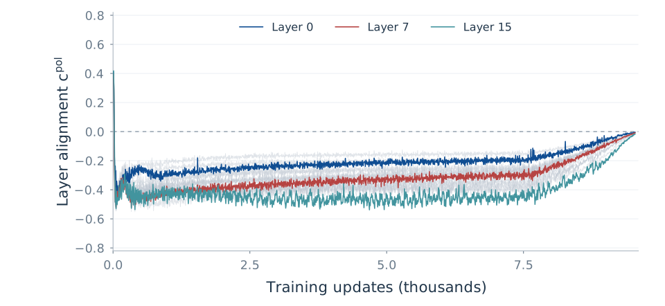
Figure 12 · Larger-scale directional evidence. Loss improves while global alignment is more negative than in the displayed 130M baseline. The lower panel includes all 16 layers and highlights three for readability. This run has no T1 probes.
The larger batch is consistent with the controlled trend, but the 130M-to-1B comparison changes several factors and does not isolate batch size. No T1 probes were collected at 1B; this run supplies directional evidence, not a test of conditional loss neutrality.
7. What survives—and why “sublates”?
Muon preserves a coherence-corrected loss‑neutral edge and changes its relation to temporal reversal. The loss identity defines T1. Polar geometry makes T2 depend on a different response. The matrix example proves separation; controlled training and LLM experiments show how it appears in practice.
At 130M scale, loss-boundary tracking coexists with weak negative alignment. The studied 1B configuration has stronger partial cancellation, still far from coherent reversal. Layerwise measurements reveal structure hidden by a global cosine. These findings give a split EoS picture: a surviving loss boundary has no universal temporal-direction signature.
That is what sublates means here: preserving an essential part of the classical picture while changing its structure. A complete stochastic perturbation-stability characterization is a different mathematical task; our loss and direction results specify the signatures actually tested along training.
Can these quantities guide learning-rate and batch-size schedules?
The learning-rate branches suggest a practical next question: could we use the measured loss balance and directional alignment to choose a schedule during training? The two quantities provide complementary information. One tells us how a candidate step trades descent against curvature; the other tells us how successive directions reinforce or partially cancel.
For the loss-side signal, define the distance from conditional balance as
\[D_b(W;\eta)=s_b^M(W;\eta)-\frac{2\rho_b(W)}{\eta}.\]By the conditional identity, negative \(D_b\) means expected descent, zero means loss neutrality, and positive \(D_b\) means an expected increase for the analyzed step. Alongside it, track \(c_k^{\mathrm{pol}}\) to describe the temporal direction response. A loss-neutral step and a nearly orthogonal next direction are separate observations, and a scheduler can use both.
Learning rate: measure how the balance moves
At selected checkpoints, a future scheduler could probe a small set of candidate learning rates and estimate their conditional loss changes. Short continuations could then show how the directional cosine responds. This follows the logic of our checkpoint intervention: starting from the same state, changing the rate can move the expected loss response across zero while later directions remain negatively aligned.
For a warmup–stable–decay (WSD) schedule, these measurements could help choose the stable-phase rate and investigate when to begin decay. A useful target might be a chosen neighborhood of the loss boundary, assessed together with the directional response and validation progress. The effective curvature depends on the candidate step itself, so each rate should be evaluated rather than obtained by treating the measured curvature as a fixed constant in the boundary equation. We have not yet established an optimal target or switching rule.
Critical batch size: locate diminishing returns
Batch size changes both the coherence of a sampled polar direction and its temporal behavior. Our controlled experiments already show that changing the batch size can reverse the order in which T1 and T2 are encountered. The coherence measurements provide another part of the picture: increasing the batch can retain more of the full-gradient descent signal.
A natural next experiment is therefore a joint learning-rate and batch-size sweep at a fixed checkpoint. For each candidate batch, measure the loss-side balance and then use short continuations to measure alignment. Compare the resulting validation improvement at matched token budgets, recording wall-clock cost as well. This would test whether larger batches continue to buy useful progress or mainly make successive updates more redundant or more strongly opposing.
In this approach, a candidate critical batch size is a region where increasing the batch yields diminishing improvement per token or per unit time. Saturation of coherence and changes in directional alignment could help identify where to look. They are diagnostic clues: the critical batch size is not defined by \(c=0\) or by T1 alone. Repeating the measurement during training could support a changing batch-size schedule jointly with the learning-rate schedule.
Measure at a checkpoint
Probe candidate rates and batches for conditional loss balance.
Follow short continuations
Track directional alignment and validation progress.
Evaluate a schedule
Compare rate and batch choices at matched budgets; repeat later in training.
This is a proposed use of the two diagnostics, rather than a scheduler already validated by our experiments. The additional momentum-Muon and AdamW runs also make the role of history clear: their persistently positive alignment motivates studying schedule targets that account for memory. The loss-boundary analysis here centers on Muon without momentum.
We can now return to the opening question. Muon retains a meaningful loss-balance edge, while its matrix geometry changes how that edge relates to consecutive directions. Understanding both sides gives us a more informative description of training—and concrete quantities with which to investigate its schedule.
Paper, code and further reading
Yanzhe Chen, Qifang Zhao, Xiaoxiao Xu, and Fanghui Liu. Muon Sublates the Edge of Stability in LLM Pretraining, arXiv v1. Code.
Background: Wu, Ma and E (2018); Cohen et al. (2021); Jordan et al., Muon; Bernstein, Deriving Muon.
For additional geometric demos: Neel Mishra, Muon Part 1 and Newton–Schulz Part 2. Our new diagrams and geometric interpolation are independently implemented; no external demo assets are embedded. The question-led exposition and figure walkthroughs take inspiration from Central Flows; expandable technical details also draw on Tri Dao’s ReplaySSM blog.